Quantitative : Discrete, Continuous
Referred to as numeric, Quantitative data have two types: Discrete and Continuos. Continuous are measurement and discrete are counts, as a general rule.
A count that can't be made precise more is discrete data. It involves integers typically. It is a discrete data which is the number of children (or pets, or adults), for instance, the reason is whole are counting by yourself, entities indvisible: 1.3 pets or 2.5 kids, you can't have it.
On the other hand, continuos data, to finer and finer levels it could reduce and could be divided. For examlple, at progressively more precise - beyond, milimiters, centimeters and meters - so height are continuos data.
Qualitative
Qualitative data is characterizes or approximates by data but properties, attributes, characteristics, etc are not measured, of phenomenon or a thin. Whereas quantitative data defines is where qualitative data describes.
Wednesday, 13 July 2016
Measures of dispersion
Standard Deviation
Within a set of data, a measure of the spread of scores are the standard deviation defines.
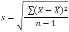
where,
 = sample mean
n = number of scores in sample.
s = sample standard deviation
 = sum of...
Within a set of data, a measure of the spread of scores are the standard deviation defines.
Formulas for the standard deviation
Sample standard deviation formula is:where,
n = number of scores in sample.
s = sample standard deviation
Measures of central tendency
Mean:
-- The mean is found when the numbers of data entries dividing and adding up all of the given data. It is also known as the average.
Example:
- the grades were as follows, the class of grade 110 math had a mathematics test recently:
78
66
82 464 / 6 = 77.3
89
75 Hence, the mean average of the class is 77.3.
+ 74
464
Median:
-- The middle number is the median. First you arrange the numbers in order from lowest. Firstly, from the lowest, in order you arrange the numbers
to highest, by crossing off the numbers until you reach the
middle then you find the middle number.
Example:
- to find the median, use the above data:
66 74 75 78 82 89\
- There is no middle number, as you can see we have two numbers What should we do?
find the average and we take the two middle numbers , ( or mean ). It is simple;
75 + 78 = 153
153 / 2 = 76.5
Hence, 76.5 is the middle number.
Mode:
-- this is the number that most often occurs.
Example:
- the following data below, find the mode:
78 56 68 92 84 76 74 56 68 66 78 72 66
65 53 61 62 78 84 61 90 87 77 62 88 81
78 is the Mode.
Sets and Venn Diagram
At the left shows overlap of two sets A and B of the Venn diagram. U is the universal set. In the center region labeled where the circles overlap is where the values that belong to both set A and set B are located. "Intersection" of the two sets is the region are called.

Videos of Shading regions Venn Diagrams
(Can only be played at google chrome)
Videos of Shading regions Venn Diagrams
(Can only be played at google chrome)
Geometric Progression
Geometric Progression, Series & Sums
Introduction
A geometric sequence is a sequence such that any element after the first is obtained by multiplying the preceding element by a constant called the common ratio which is denoted by r. The common ratio (r) is obtained by dividing any term by the preceding term, i.e.,| where | r | common ratio |
| a1 | first term | |
| a2 | second term | |
| a3 | third term | |
| an-1 | the term before the n th term | |
| an | the n th term |
For example, the sequence 1, 3, 9, 27, 81 is a geometric sequence. Note that after the first term, the next term is obtained by multiplying the preceding element by 3.
The geometric sequence has its sequence formation:
To find the nth term of a geometric sequence we use the formula:
| where | r | common ratio |
| a1 | first term | |
| an-1 | the term before the n th term | |
| n | number of terms |
Arithmetic Progression
Arithmetic Progression
An arithmetic progression is a sequence of numbers such that the difference of any two successive members is a constant.For example, the sequence 1, 2, 3, 4, ... is an arithmetic progression with common difference 1.
Second example: the sequence 3, 5, 7, 9, 11,... is an arithmetic progression
with common difference 2.
Third example: the sequence 20, 10, 0, -10, -20, -30, ... is an arithmetic progression
with common difference -10.
Notation
We denote by d the common difference.By an we denote the n-th term of an arithmetic progression.
By Sn we denote the sum of the first n elements of an arithmetic series.
Arithmetic series means the sum of the elements of an arithmetic progression.
Properties
a1 + an = a2 + an-1 = ... = ak + an-k+1
and
an = ½(an-1 + an+1)
Sample: let 1, 11, 21, 31, 41, 51... be an arithmetic progression.
51 + 1 = 41 + 11 = 31 + 21
and
11 = (21 + 1)/2
21 = (31 + 11)/2...
If the initial term of an arithmetic progression is a1 and the common difference of successive members is d, then the n-th term of the sequence is given by
an = a1 + (n - 1)d, n = 1, 2, ...
The sum S of the first n numbers of an arithmetic progression is given by the formula:
S = ½(a1 + an)n
where a1 is the first term and an the last one.
or
S = ½(2a1 + d(n-1))n
Linear Inequalities
Linear inequalities in general dimensions
In Rn linear inequalities are the expressions that may be written in the formor

 and b a constant real number.
More concretely, this may be written out as


 are called the unknowns, and
  are called the coefficients.
Alternatively, these may be written as
or

That is


Systems of linear inequalities
A system of linear inequalities is a set of linear inequalities in the same variables:
 are the unknowns,
  are the coefficients of the system, and
  are the constant terms.
This can be concisely written as the matrix inequality

In the above systems both strict and non-strict inequalities may be used.
- Not all systems of linear inequalities have solutions.
Tuesday, 12 July 2016
Linear programming (LP) (also called linear optimization) is a method to achieve the best outcome (such as maximum profit or lowest cost) in a mathematical model whose requirements are represented by linear relationships. Linear programming is a special case of mathematical programming (mathematical optimization).
More formally, linear programming is a technique for the optimization of a linear objective function, subject to linear equality and linear inequality constraints. Its feasible region is a convex polytope, which is a set defined as the intersection of finitely many half spaces, each of which is defined by a linear inequality. Its objective function is a real-valued affine (linear) function defined on this polyhedron. A linear programming algorithm finds a point in the polyhedron where this function has the smallest (or largest) value if such a point exists.
Linear programs are problems that can be expressed in canonical form as

- where x represents the vector of variables (to be determined), c and b are vectors of (known) coefficients, A is a (known) matrix of coefficients, and
is the matrix transpose. The expression to be maximized or minimized is called the objective function (cTx in this case). The inequalities Ax ≤ b and x ≥ 0 are the constraints which specify a convex polytope over which the objective function is to be optimized. In this context, two vectors are comparable when they have the same dimensions. If every entry in the first is less-than or equal-to the corresponding entry in the second then we can say the first vector is less-than or equal-to the second vector.
Wednesday, 8 June 2016
LOGARITHM
WHEN WE ARE GIVEN the base 2, for example, and exponent 3, then we can evaluate 23.
23 = 8.
Inversely, if we are given the base 2 and its power 8 --
2? = 8
-- then what is the exponent that will produce 8?
That exponent is called a logarithm. We call the exponent 3 the logarithm of 8 with base 2. We write
3 = log28.
We write the base 2 as a subscript. 3 is the exponent to which 2 must be raised to produce 8.
A logarithm is an exponent.
Since
104 = 10,000
then
log1010,000 = 4.
"The logarithm of 10,000 with base 10 is 4."
4 is the exponent to which 10 must be raised to produce 10,000.
"104 = 10,000" is called the exponential form.
"log1010,000 = 4" is called the logarithmic form.
Here is the definition:
logbx = n means bn = x.
That base with that exponent produces x.
Example 1. Write in exponential form: log232 = 5.
Answer. 25 = 32.
| Example 2. Write in logarithmic form: 4−2 = | 1 16 |
. |
| Answer. log4 | 1 16 |
= −2. |
Problem 1. Which numbers have negative logarithms?
To see the answer, pass your mouse over the colored area.
To cover the answer again, click "Refresh" ("Reload").
Do the problem yourself first!
To cover the answer again, click "Refresh" ("Reload").
Do the problem yourself first!
Proper fractions.
Example 3. Evaluate log81.
Answer. 8 to what exponent produces 1? 80 = 1.
log81 = 0.
We can observe that, in any base, the logarithm of 1 is 0.
logb1 = 0
Example 4. Evaluate log55.
Answer. 5 with what exponent will produce 5? 51 = 5. Therefore,
log55 = 1.
In any base, the logarithm of the base itself is 1.
logbb = 1
Example 5 . log22m = ?
Answer. 2 raised to what exponent will produce 2m ? m, obviously.
log22m = m.
The following is an important formal rule, valid for any base b:
logbbx = x
This rule embodies the very meaning of a logarithm. x -- on the right -- is the exponent to which the base b must be raised to produce bx.
The rule also shows that the exponential function bx is the inverse of the function logbx. We will see this in the following Topic.
| Example 6 . Evaluate log3 | 1 9 |
. |
| Answer. | 1 9 |
is equal to 3 with what exponent? | 1 9 |
= 3−2. |
| log3 | 1 9 |
= | log33−2 = −2. |
Compare the previous rule.
Example 7. log2 .25 = ?
Answer. .25 = ¼ = 2−2. Therefore,
log2 .25 = log22−2 = −2.
Laws of Indices
When working with indices, there are three rules that should be used:
When m and n is positive integers,
This is the definition of an logical consequences, these three are the results, but formal proof are really needed.With particular examples as below, you can 'verify' them, but this are not the proof.| 1. | am × an = am + n | ||||
|---|---|---|---|---|---|
| 2. | am ÷ an = am – n or |
| = am – n (m ≥ n) | ||
| 3. | (am)n = am × n |
| 27× 23 | = | (2 × 2 × 2 × 2 × 2 × 2 × 2) × (2 × 2 × 2) | |
| = | 2 × 2 × 2 × 2 × 2 × 2 × 2 × 2 × 2 × 2 | ||
| = | 210 | (here m = 7, n = 3 and m + n = 10) |
| 27 ÷ 23 | = |
| |||
| = | 2 × 2 × 2 × 2 | ||||
| = | 24 | (again m = 7, n = 3 and m – n = 4) |
| (27)3 | = | 27 × 27 × 27 | |
| = | 221 | (using rule 1) (again m = 7, n = 3 and m × n = 21) |
Proof
| am × an | = | a × a × ... × a
|
× | a × a × ... × a
|
||||||||||
| = | a × a × ... × a × a × a × ... × a
|
|||||||||||||
| = | am+n | |||||||||||||


Using rule 2 we can see an important result:
| = xn – n = x0 | ||||
| but |
| = 1, | so |
x0 = 1
This is true for any non-zero value of x, so, for example, 30 = 1, 270 = 1 and 10010 = 1.
Subscribe to:
Comments (Atom)